How To Create A Data Model In Python

Create a model to predict house prices using Python

Hey there ,

Last time we saw how to do logistic regression on titanic dataset which many professional data scientist would say is the first step towards doing a data science project. If you didn't you can find it here ,

So , I'm assuming you know the basic libraries of python (if not then go through the above tutorial). we are going to use the same libraries which we used last time with the addition of seaborn which is another built in python library used to do data representation.

Last time , we did for a dataset which had data about Titanic passengers , we knew what happened to Titanic and we didn't need to skim through the dataset. But most of the times , data scientists are given data which are unknown to them. It is very important to know in depth about the data.

So far so good , Today we are going to work on a dataset which consists information about the location of the house , price and other aspects such as square feet etc. When we work on these sort of data , we need to see which column is important for us and which is not. Our main aim today is to make a model which can give us a good prediction on the price of the house based on other variables. We are going to use Linear Regression for this dataset and see if it gives us a good accuracy or not.

What is good accuracy ? Well , it depends on what sort of data we are working with , for a credit risk data an accuracy of 80% may not be good enough but for a data using NLP it would be good. So we can't actually define "good accuracy" but anything above 85% is good. Our aim on this dataset is to achieve an accuracy score of 85%+

Let's begin , The data and the code can be found on my github link

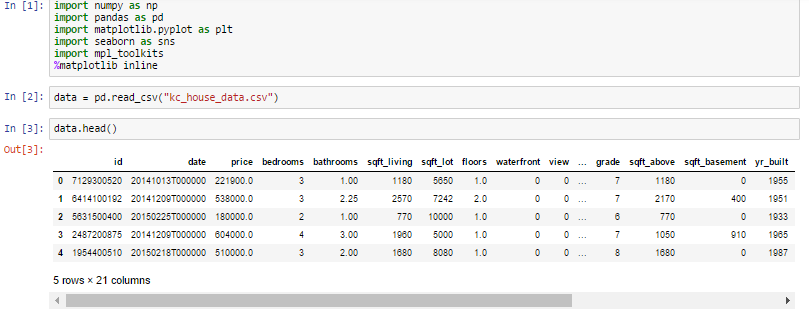
First thing first , we import our libraries and dataset and then we see the head of the data to know how the data looks like and use describe function to see the percentile's and other key statistics.

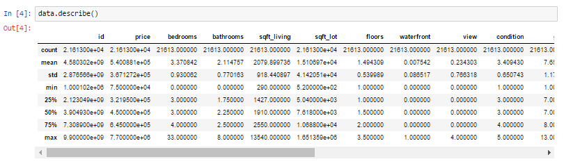
Starting , by importing libraries and reading dataset

What can we infer from the above describe function ?

Look at the bedroom columns , the dataset has a house where the house has 33 bedrooms , seems to be a massive house and would be interesting to know more about it as we progress.
Maximum square feet is 13,450 where as the minimum is 290. we can see that the data is distributed.

Similarly , we can infer so many things by just looking at the describe function.

Now , we are going to see some visualization and also going to see how and what can we infer from visualization.

Which is the most common house (Bedroom wise) ?

Let's see which is most common bedroom number. You may wonder why is it important ? Let's look at this problem from a builder's perspective, sometimes it's important for a builder to see which is the highest selling house type which enables the builder to make house based on that. Here in India , for a good locality a builder opts to make houses which are more than 3 bedrooms which attracts the higher middle class and upper class section of the society.

Let's see how this pans out for this data ?

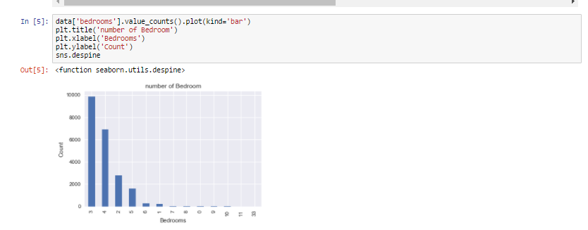
As we can see from the visualization 3 bedroom houses are most commonly sold followed by 4 bedroom. So how is it useful ? For a builder having this data , He can make a new building with more 3 and 4 bedroom's to attract more buyers.

So now we know that 3 and 4 bedroom's are highest selling. But at which locality ?

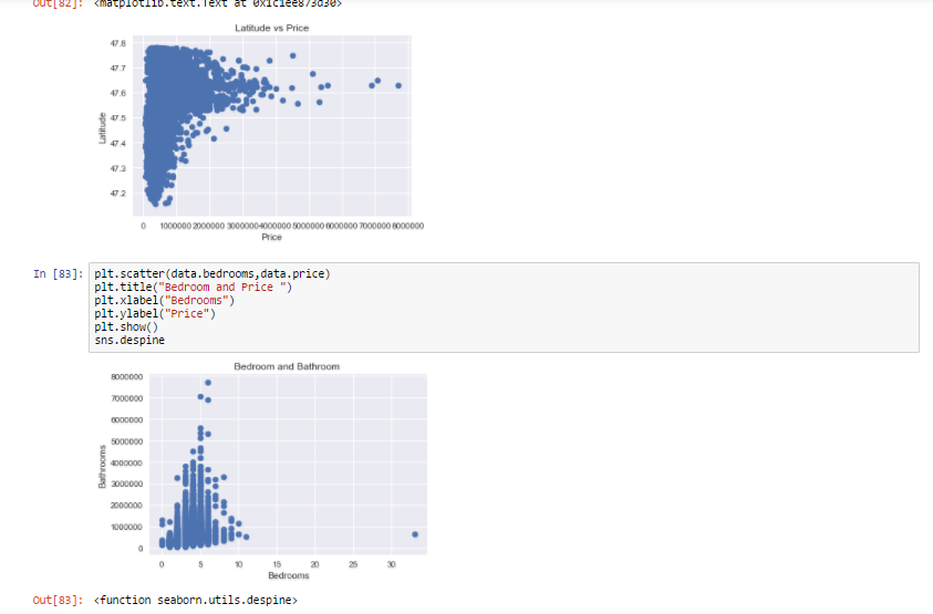
Visualizing the location of the houses based on latitude and longitude.

So according to the dataset , we have latitude and longitude on the dataset for each house. We are going to see the common location and how the houses are placed.

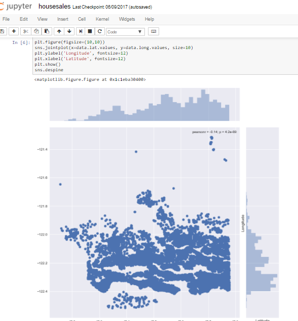
We use seaborn , and we get his beautiful visualization. Joinplot function helps us see the concentration of data and placement of data and can be really useful. Let us see what we can infer from this visualization. For latitude between -47.7 and -48.8 there are many houses , which would mean that maybe it's an ideal location isn't it ? But when we talk about longitude we can see that concentration is high between -122.2 to -122.4. Which would mean that most of the buy's has been for this particular location.

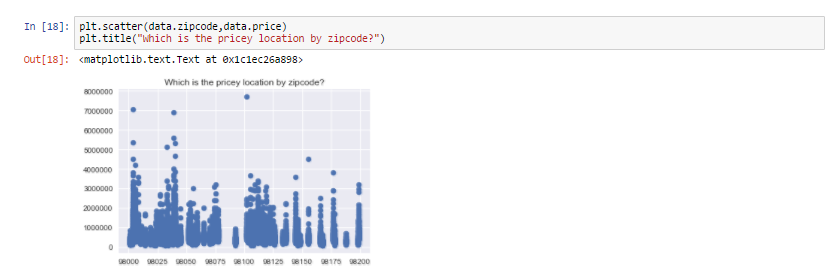
How common factors are affecting the price of the houses ?

We saw the common locations and now we're going to see few common factors affecting the prices of the house and if so ? then by how much ?

Let us start with , If price is getting affecting by living area of the house or not ?

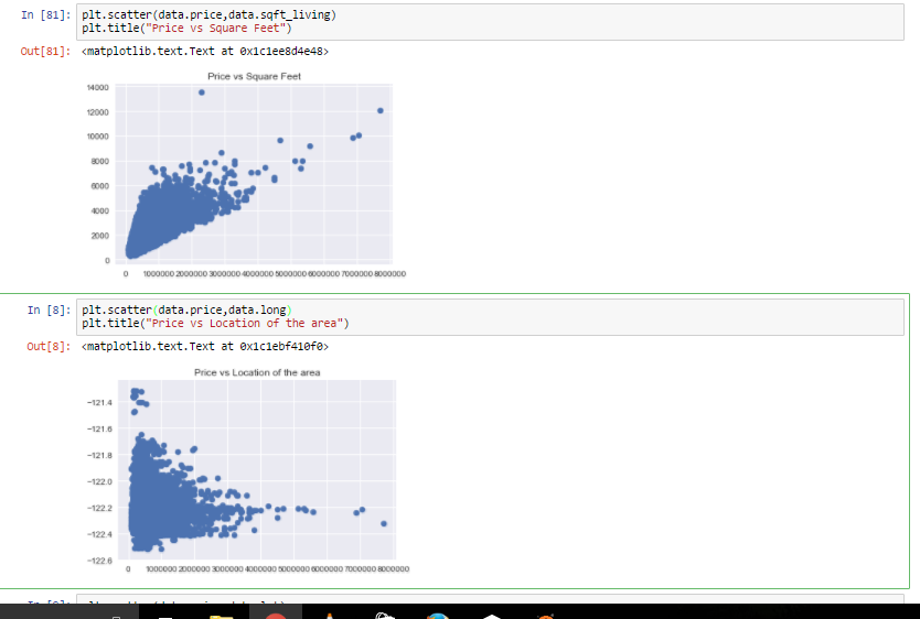
Price vs Square feet and Price vs Longitude

The plot that we used above is called scatter plot , scatter plot helps us to see how our data points are scattered and are usually used for two variables. From the first figure we can see that more the living area , more the price though data is concentrated towards a particular price zone , but from the figure we can see that the data points seem to be in linear direction. Thanks to scatter plot we can also see some irregularities that the house with the highest square feet was sold for very less , maybe there is another factor or probably the data must be wrong. The second figure tells us about the location of the houses in terms of longitude and it gives us quite an interesting observation that -122.2 to -122.4 sells houses at much higher amount.

We can see more factors affecting the price

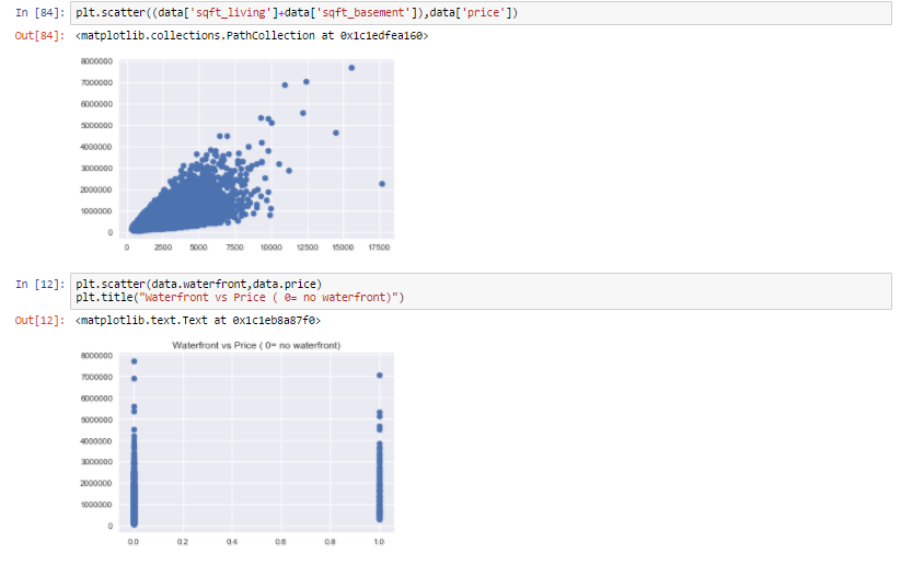
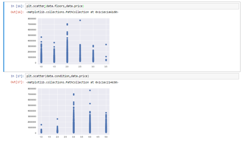
Total sqft including basement vs price and waterfront vs price

As we can see from all the above representation that many factors are affecting the prices of the house , like square feet which increases the price of the house and even location influencing the prices of the house.

Now that we are familiar with all these representation and can tell our own story let us move and create a model to which would predict the price of the house based upon the other factors such as square feet , water front etc . We are going to see what is linear regression and how do we do it ?

Linear Regression :-

In easy words a model in statistics which helps us predicts the future based upon past relationship of variables. So when you see your scatter plot being having data points placed linearly you know regression can help you!

Regression works on the line equation , y=mx+c , trend line is set through the data points to predict the outcome.

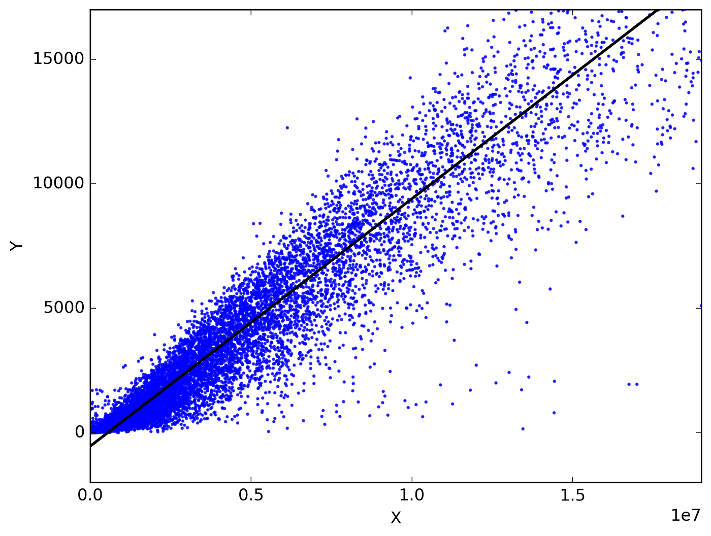
The variable we are predicting is called the criterion variable and is referred to as Y. The variable we are basing our predictions on is called the predictor variable and is referred to as X. When there is only one predictor variable, the prediction method is called Simple Regression. and if multiple predictor variable are present then multiple regression.

Let's look at the code ,

Linear regression on the data to predict prices

We use train data and test data , train data to train our machine and test data to see if it has learnt the data well or not. Before anything , I want everyone to remember that the machine is the student and train data is the syllabus and test data is the exam. we see how much the machine has scored and if it scores well are model is successful.

So what did we do ? Let's go step by step.

We import our dependencies , for linear regression we use sklearn (built in python library) and import linear regression from it.
We then initialize Linear Regression to a variable reg.
Now we know that prices are to be predicted , hence we set labels (output) as price columns and we also convert dates to 1's and 0's so that it doesn't influence our data much . We use 0 for houses which are new that is built after 2014.
We again import another dependency to split our data into train and test.
I've made my train data as 90% and 10% of the data to be my test data , and randomized the splitting of data by using random_state.
So now , we have train data , test data and labels for both let us fit our train and test data into linear regression model.
After fitting our data to the model we can check the score of our data ie , prediction. in this case the prediction is 73%

The accuracy of the model is lower than our aim of 85. So how do we achieve that 85% target ?

We use a different method , which is very important for weak prediction models such as this.

This might seem to be a bit advanced but if understood is a really brilliant tool to enable better predictions.

For building a prediction model , many experts use gradient boosting regression , so what is gradient boosting ? It is a machine learning technique for regression and classification problems, which produces a prediction model in the form of an ensemble of weak prediction models, typically decision trees.

Now to make it easy , remember how we mapped machine as a student , train data as the syllabus and test data as the exam. let's try to understand gradient boosting method using the same. So , let's analyse why our student (machine) didn't get above 85% ? there could be many reasons few such reasons could be :-

Our student forgot few of the topics before giving the exam , Similarly data read by machine can be lost.
It could be a weak learner who doesn't learn by reading but needs visualization. Our machine can be a weak learner and may require decision tree.
Even after using newer technique our student may not remember the syllabus so we give our student time to read and understand. Similarly for machine .

Hence for all this problems there is one fix , Gradient descent boosting.

This link gives an in depth understanding about gradient boosting algorithm.

Gradient boosting graph for understanding

Let's look at how we do that and then we can go in depth and understand what is happening.

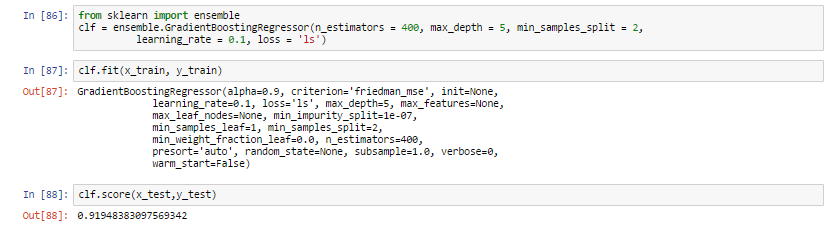
We first import the library from sklearn ( trust me , it is the best library for all statistical related models)
We create a variable where we define our gradient boosting regressor and set parameters to it , here

n_estimator — The number of boosting stages to perform. We should not set it too high which would overfit our model.

max_depth — The depth of the tree node.

learning_rate — Rate of learning the data.

loss — loss function to be optimized. 'ls' refers to least squares regression

minimum sample split — Number of sample to be split for learning the data

3. We then fit our training data into the gradient boosting model and check for accuracy

4. We got an accuracy of 91.94% which is amazing!

We can see that for weak predictions gradient boosting does the trick for the same train and test data.

Check this link out for more about gradient boosting regressor

We got what we wanted! an accuracy score of 91.94%. Apply this technique on various other datasets and post your results. Try to put random seeds and check if it changes the accuracy of the data or not! Let me know if it does. Thank you for giving it a read!

Hope you enjoyed it! Bye for now , will be back with more models and contents! Please share and recommend to your friends.

Update : The code for this can be found on https://github.com/Shreyas3108/house-price-prediction